About component-wise boosting

Instead of getting huge predictive power, model-based (or component-wise) boosting aggregates statistical models to maintain interpretability. This is done by restricting the used base learners to be linear in the parameters. This is important in terms of parameter estimation. For instance, having a base learner \(b_j(x, \theta^{[m]})\) of a feature \(x\) with a corresponding parameter vector \(\theta^{[m]}\) and another base learner \(b_j\) of the same type but with a different parameter vector \(\theta^{[m^\prime]}\), then it is possible, due to linearity, to combine those two learners to a new one, again, of the same type: \[ b_j(x, \theta^{[m]}) + b_j(x, \theta^{[m^\prime]}) = b_j(x, \theta^{[m]} + \theta^{[m^\prime]}) \] Instead of boosting trees like xgboost, component-wise boosting is (commonly) used with statistical models to construct an interpretable model with inherent feature selection.

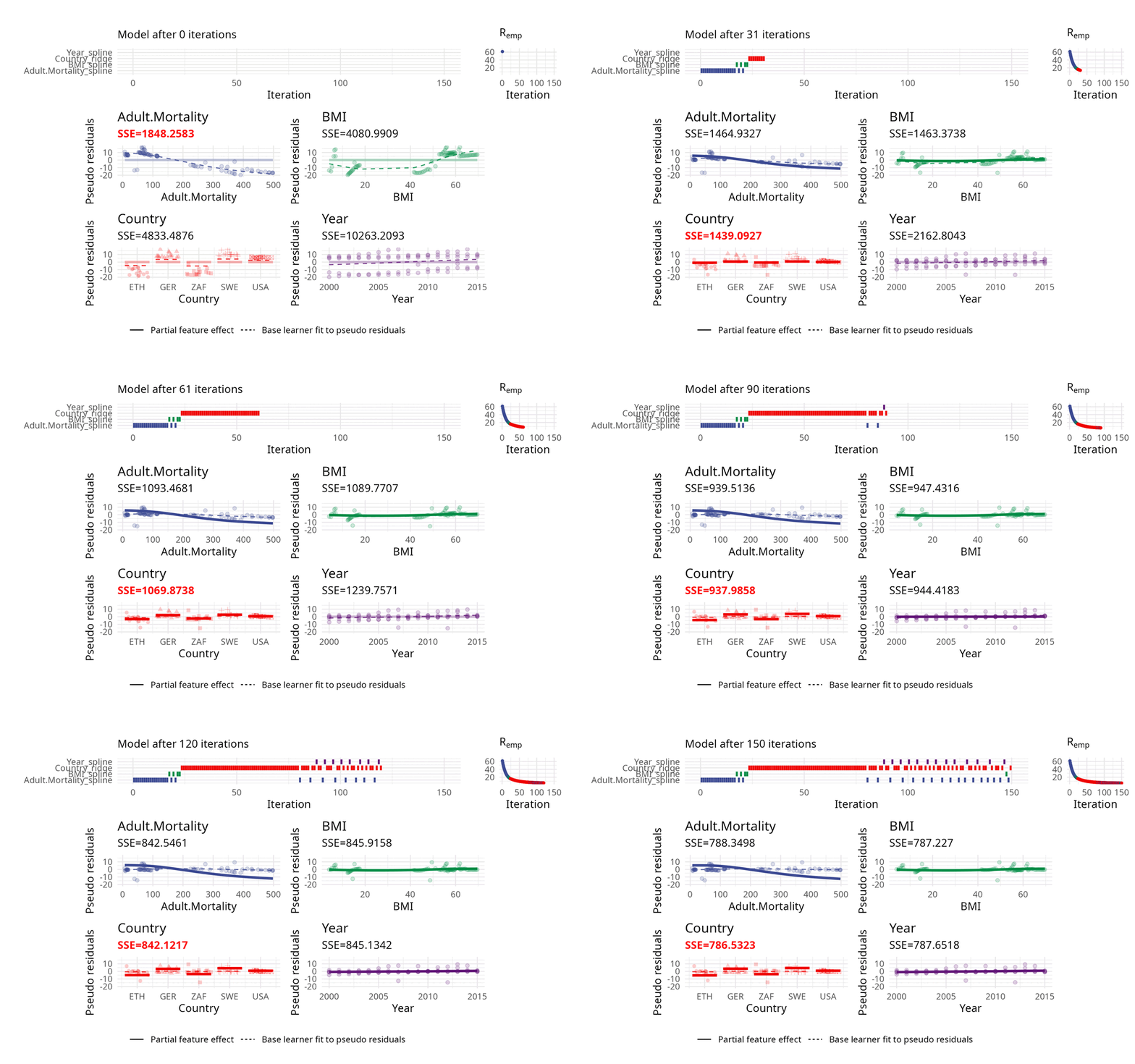
The usual way of choosing base learners is done by a greedy search. Therefore, in each iteration, all base learners are fitted to the so-called pseudo residuals that act as a kind of model error and in which direction the model should evolve to become better. A new base learner is then selected by choosing the base learner with the best fit to these pseudo residuals.

The illustration above uses three base learners \(b_1\), \(b_2\), and \(b_3\). You can think of each base learner as a wrapper around a feature which represents the effect of that feature. Hence, selecting a base learner more frequently than another one can indicate a higher importance.

\[ \begin{align} \text{Iteration 1:} \ &\hat{f}^{[1]}(x) = f_0 + \beta b_3(x_3, \theta^{[1]}) \\ \text{Iteration 2:} \ &\hat{f}^{[2]}(x) = f_0 + \beta b_3(x_3, \theta^{[1]}) + \beta b_3(x_3, \theta^{[2]}) \\ \text{Iteration 3:} \ &\hat{f}^{[3]}(x) = f_0 + \beta b_3(x_3, \theta^{[1]}) + \beta b_3(x_3, \theta^{[2]}) + \beta b_1(x_1, \theta^{[3]}) \end{align} \] Using the linearity of the base learners allows to aggregate \(b_3\): \[ \hat{f}^{[3]}(x) = f_0 + \beta \left( b_3(x_3, \theta^{[1]} + \theta^{[2]}) + b_1(x_1, \theta^{[3]}) \right) \]

This simple example illustrates some strength of component-wise boosting. For example, an inherent variable selection or the estimation of partial feature effects. Further, component-wise boosting is an efficient approach to get fit to high-dimensional feature spaces \(p \gg n\).