Decompose the predicted value based on the given features
Source:R/plot_ind_contr.R
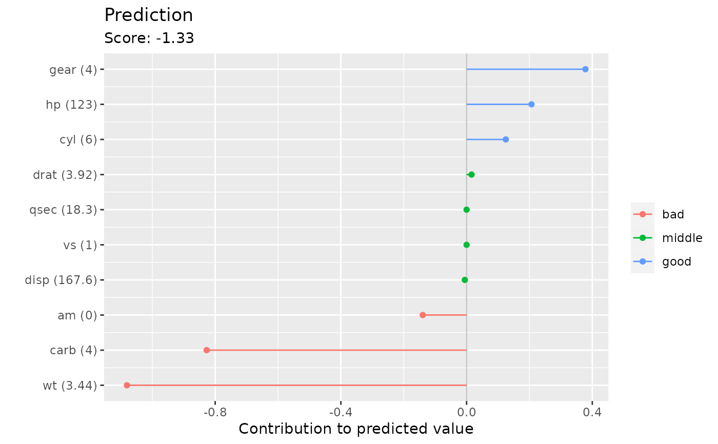
plotIndividualContribution.RdThis function visualizes the contribution of each feature regarding the predicted value.
By default, multiple base learners defined on one feature are aggregated. If you
want to show the contribution of single base learner, then set aggregate = FALSE.
Arguments
- cboost
- newdata
(
data.frame())
Data frame containing exactly one row holding the new observations.- aggregate
(
logical(1L))
Number of colored base learners added to the legend.- colbreaks
(
numeric())
Breaks to visualize/highlight different predicted values. Default creates different colors for positive and negative score values. If set toNULLno coloring is applied.- collabels
(
character(length(colbreaks) - 1))
Labels for the color breaks. If set toNULLintervals are used as labels.- nround
(
integer(1L))
Digit passed to round for labels (default isnround = 2L).- offset
(
logical(1L))
Flag to indicate whether the offset should be added to the figure or not.
Examples
dat = mtcars
fnum = c("cyl", "disp", "hp", "drat", "wt", "qsec")
fcat = c("vs", "am", "gear", "carb")
for (fn in fcat) dat[[fn]] = as.factor(dat[[fn]])
cboost = Compboost$new(data = dat, target = "mpg",
loss = LossQuadratic$new())
for (fn in fnum) cboost$addComponents(fn, df = 3)
for (fn in fcat) cboost$addBaselearner(fn, "ridge", BaselearnerCategoricalRidge)
cboost$train(500L)
#> 1/500 risk = 16
#> 12/500 risk = 7.9
#> 24/500 risk = 4.6
#> 36/500 risk = 3.4
#> 48/500 risk = 3
#> 60/500 risk = 2.7
#> 72/500 risk = 2.6
#> 84/500 risk = 2.6
#> 96/500 risk = 2.5
#> 108/500 risk = 2.5
#> 120/500 risk = 2.4
#> 132/500 risk = 2.4
#> 144/500 risk = 2.4
#> 156/500 risk = 2.3
#> 168/500 risk = 2.3
#> 180/500 risk = 2.3
#> 192/500 risk = 2.3
#> 204/500 risk = 2.3
#> 216/500 risk = 2.2
#> 228/500 risk = 2.2
#> 240/500 risk = 2.2
#> 252/500 risk = 2.2
#> 264/500 risk = 2.2
#> 276/500 risk = 2.2
#> 288/500 risk = 2.1
#> 300/500 risk = 2.1
#> 312/500 risk = 2.1
#> 324/500 risk = 2.1
#> 336/500 risk = 2.1
#> 348/500 risk = 2.1
#> 360/500 risk = 2.1
#> 372/500 risk = 2.1
#> 384/500 risk = 2.1
#> 396/500 risk = 2
#> 408/500 risk = 2
#> 420/500 risk = 2
#> 432/500 risk = 2
#> 444/500 risk = 2
#> 456/500 risk = 2
#> 468/500 risk = 2
#> 480/500 risk = 2
#> 492/500 risk = 2
#>
#>
#> Train 500 iterations in 0 Seconds.
#> Final risk based on the train set: 2
#>
cbreaks = c(-Inf, -0.1, 0.1, Inf)
clabs = c("bad", "middle", "good")
plotIndividualContribution(cboost, dat[10, ], colbreaks = cbreaks,
collabels = clabs)
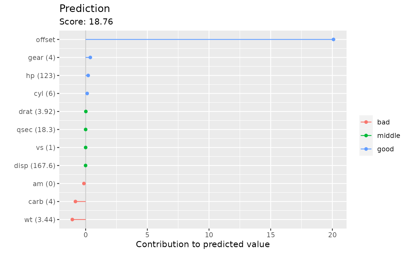 plotIndividualContribution(cboost, dat[10, ], offset = FALSE,
colbreaks = cbreaks, collabels = clabs)
plotIndividualContribution(cboost, dat[10, ], offset = FALSE,
colbreaks = cbreaks, collabels = clabs)