[Compboost] contains two mlr3 learners
for regression regr.compboost and binary classification
classif.compboost. See https://mlr3.mlr-org.com/ For an
introduction to mlr3. Here, we show the two learners in
small examples.
Regression
As task, we use the Boston housing task that is accessible via
tsk("boston_housing"):
library(mlr3)

task = tsk("boston_housing")
task
#> <TaskRegr:boston_housing> (506 x 19): Boston Housing Prices
#> * Target: medv
#> * Properties: -
#> * Features (18):
#>   - dbl (13): age, b, cmedv, crim, dis, indus, lat, lon, lstat, nox,
#>     ptratio, rm, zn
#>   - int (3): rad, tax, tract
#>   - fct (2): chas, town
The key regr.compboost gives the regression learner:
lcb = lrn("regr.compboost")
lcb$param_set
#> <ParamSet>
#>                    id    class lower upper nlevels default     parents  value
#>  1:       baselearner ParamFct    NA    NA       3  spline             spline
#>  2:          bin_root ParamInt     0   Inf     Inf       0
#>  3:            degree ParamInt     1   Inf     Inf       3 baselearner
#>  4:                df ParamDbl     1   Inf     Inf       5                  5
#>  5:            df_cat ParamDbl     1   Inf     Inf       2                  2
#>  6:       differences ParamInt     1   Inf     Inf       2 baselearner
#>  7:        early_stop ParamLgl    NA    NA       2   FALSE              FALSE
#>  8:     eps_for_break ParamDbl  -Inf   Inf     Inf       0  early_stop
#>  9:      interactions ParamUty    NA    NA     Inf
#> 10:        iterations ParamInt     1   Inf     Inf     100                100
#> 11: just_interactions ParamLgl    NA    NA       2   FALSE              FALSE
#> 12:     learning_rate ParamDbl     0   Inf     Inf    0.05
#> 13:              loss ParamUty    NA    NA     Inf
#> 14:          loss_oob ParamUty    NA    NA     Inf          early_stop
#> 15:           n_knots ParamInt     1   Inf     Inf      20 baselearner
#> 16:      oob_fraction ParamDbl     0     1     Inf     0.3
#> 17:         optimizer ParamUty    NA    NA     Inf
#> 18:          patience ParamInt     1   Inf     Inf       5  early_stop
#> 19:       show_output ParamLgl    NA    NA       2   FALSE              FALSE

lcb$train(task)
lcb$model
#>
#>
#> Component-Wise Gradient Boosting
#>
#> Target variable: medv
#> Number of base-learners: 18
#> Learning rate: 0.05
#> Iterations: 100
#>
#> Offset: 22.5328
#>
#> LossQuadratic: L(y,x) = 0.5 * (y - f(x))^2
The most important features of Compboost can be
controlled via the parameters. For example, using early stopping
requires to set the value oob_fraction to a number bigger
than 0. Just in this case, the learner can be trained with early
stopping:
lcb = lrn("regr.compboost", early_stop = TRUE)
lcb$train(task)
#> Error in get_private(learner)$.train(task): `oob_fraction > 0` required for early stopping.

lcb = lrn("regr.compboost", oob_fraction = 0.3, early_stop = TRUE)
lcb$train(task)
head(lcb$model$logs)
#>   _iterations oob_risk time  baselearner train_risk
#> 1           0       NA   NA    intercept   40.37947
#> 2           1 41.06313    0 cmedv_spline   36.45684
#> 3           2 37.07316  358 cmedv_spline   32.91667
#> 4           3 33.47867  683 cmedv_spline   29.72167
#> 5           4 30.24079  995 cmedv_spline   26.83817
#> 6           5 27.32444 1314 cmedv_spline   24.23582
Binary classification
Binary classification works in the same way. We use the
spam data set for the demo:
task = tsk("spam")
task
#> <TaskClassif:spam> (4601 x 58): HP Spam Detection
#> * Target: type
#> * Properties: twoclass
#> * Features (57):
#>   - dbl (57): address, addresses, all, business, capitalAve,
#>     capitalLong, capitalTotal, charDollar, charExclamation, charHash,
#>     charRoundbracket, charSemicolon, charSquarebracket, conference,
#>     credit, cs, data, direct, edu, email, font, free, george, hp, hpl,
#>     internet, lab, labs, mail, make, meeting, money, num000, num1999,
#>     num3d, num415, num650, num85, num857, order, original, our, over,
#>     parts, people, pm, project, re, receive, remove, report, table,
#>     technology, telnet, will, you, your
Then, the usual methods and fields are accessible:
Using compboost in parallel
The parallel execution in compboost is controlled by the
optimizers. With mlr3, optimizers can defined in the
construction of the learner. Thus, if compboost should be run in
parallel, define an optimizer in advance and use it in the
construction:
lcb$timings["train"]
#> train
#> 5.858

lcb_2c = lrn("classif.compboost", iterations = 500L, optimizer = OptimizerCoordinateDescent$new(2))
lcb_2c$train(task)
lcb_2c$timings["train"]
#> train
#>  3.26
Using different losses
As for the parallel execution, losses can be defined by the
loss parameter value in the construction:
task = tsk("boston_housing")
lcb_quantiles = lrn("regr.compboost", loss = LossQuantile$new(0.1))
lcb_quantiles$train(task)
lcb_quantiles$predict(task)
#> <PredictionRegr> for 506 observations:
#>     row_ids truth response
#>           1  24.0 13.94270
#>           2  21.6 13.88014
#>           3  34.7 13.76084
#> ---
#>         504  23.9 13.94210
#>         505  22.0 13.89905
#>         506  11.9 13.62323
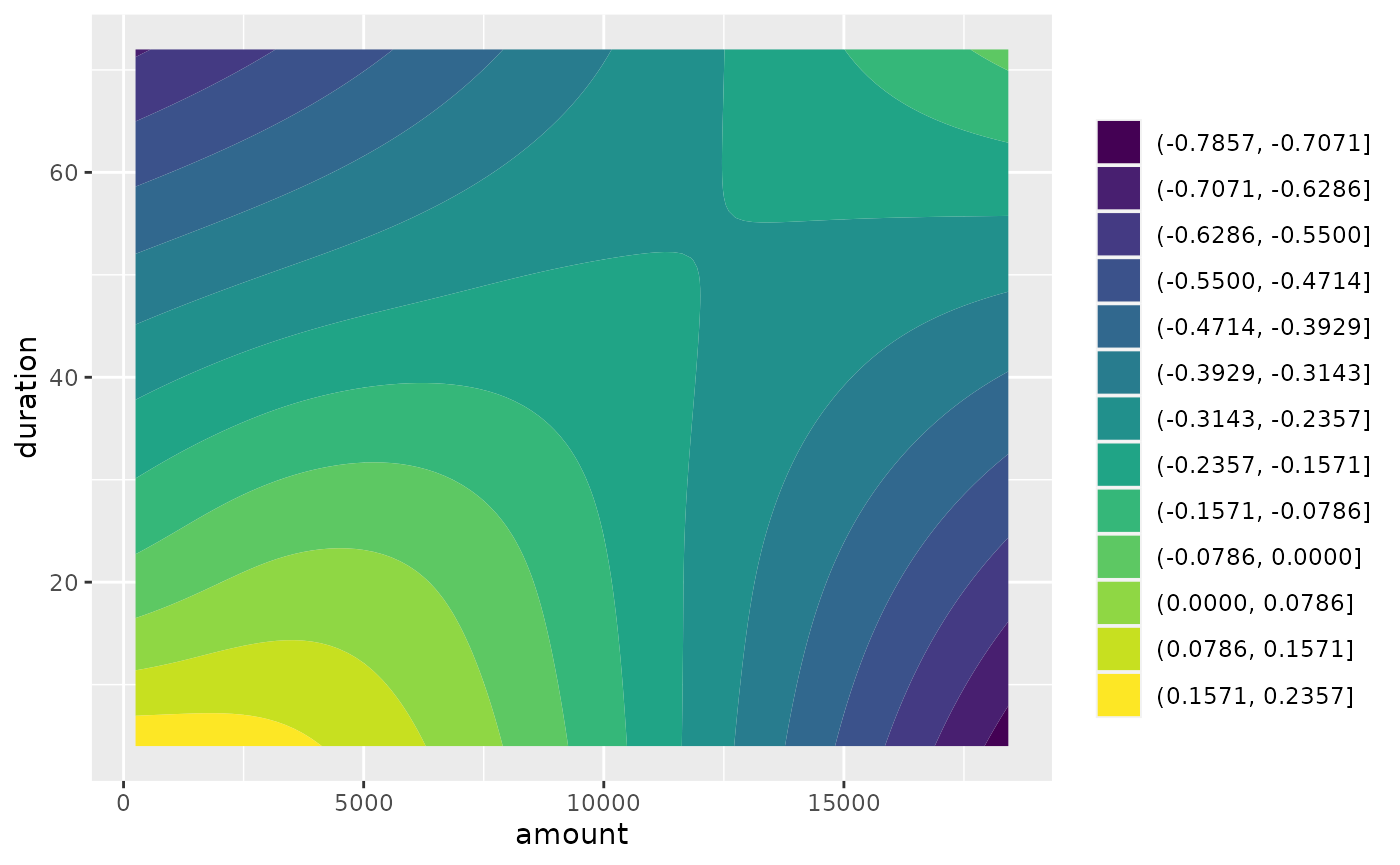
Adding interactions
Interactions can be added in the constructor by specifying a
data.frame with columns feat1 and
feat2. For each row, one row-wise tensor product base
learner is added to the model:
task = tsk("german_credit")

ints = data.frame(feat1 = c("age", "amount"), feat2 = c("job", "duration"))
ints
#>    feat1    feat2
#> 1    age      job
#> 2 amount duration

set.seed(31415)
l = lrn("classif.compboost", interactions = ints)
l$train(task)
l$importance()
#>              baselearner risk_reduction
#> 2           status_ridge     0.02703527
#> 1 amount_duration_tensor     0.01305659
plotTensor(l$model, "amount_duration_tensor")
Use early stopping
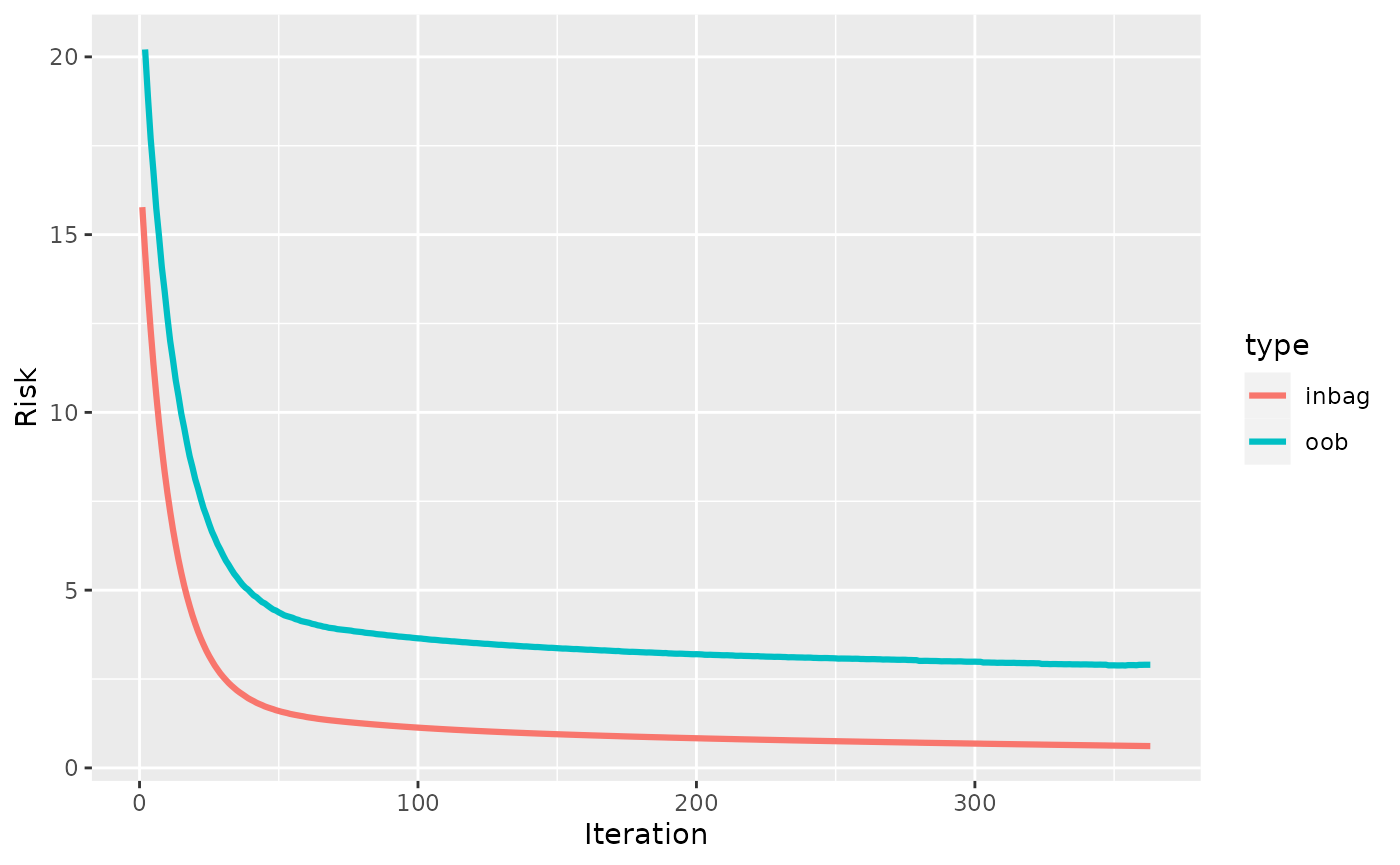
Early stopping is also controlled by the constructor. Use
early_stop = TRUE to use early stopping with the default
values patience = 5 and eps_for_break = 0 (see
?LoggerOobRisk). In compboost, early stopping
requires a validation set and hence to set
oob_fraction > 0:
task = tsk("mtcars")

set.seed(314)
l = lrn("regr.compboost", early_stop = TRUE, oob_fraction = 0.3, iterations = 1000)
l$train(task)
plotRisk(l$model)
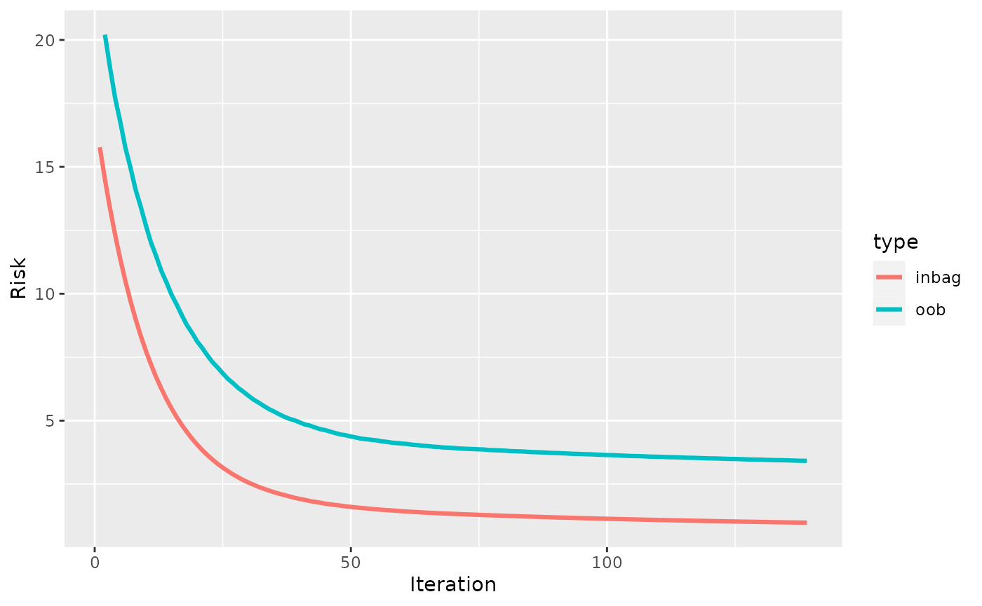
A more aggressive early stopping is achieved by setting
patience = 1:
set.seed(314)
l = lrn("regr.compboost", early_stop = TRUE, oob_fraction = 0.3, iterations = 1000,
  patience = 1)
l$train(task)
plotRisk(l$model)
Though, this is not recommended as it can stop too early without
reaching the best validation risk. Note that
oob_fraction > 0 must be true to use early stopping:
l = lrn("regr.compboost", early_stop = TRUE)
l$train(task)
#> Error in get_private(learner)$.train(task): `oob_fraction > 0` required for early stopping.